Advanced Example STCyclotron
Responsible Geant4 Collaborator: Susanna Guatelli, Centre For Medical Radiation Physics, Wollongong University, Australia.
Developers: F. Poignant (IN2P3, France), S. Penfold (University of Adelaide, Australia), P. Takhar and J. Asp (SAHMRI, Adelaide).
Short description
The STCyclotron example simulates the solid target of the South Australian Health and Medical Research Institute (SAHMRI), Adelaide, South Australia. The simulation aims at modelling the production of radio-isotopes and undesired by-products. An example of the use of the Geant4 STCyclotron application in research is available in F. Poignant, S. Penfold, J. Asp, P. Takhar, P. Jackson, Geant4 simulation of cyclotron radioisotope production in a solid target, Physica Medica, Volume 32, Issue 5, 2016, Pages 728-734, ISSN 1120-1797.
For more information on the simulated cyclotron, please visit: https://www.comecer.com/new-research-study-simulation-solid-target-performance.
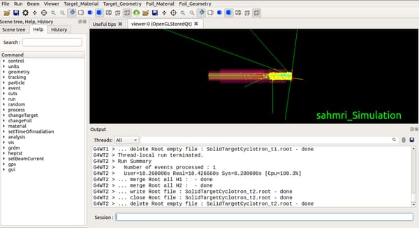
The reader should refer to the README file to have information on how to run this example. Figure 1 shows the visualisation of the simulation set-up.
Simulation results
ROOT file (STCyclotron.root). This ROOT file is generated as output of the simulation and contains a list of histograms representing the following data:
- 1D histograms:
- The energy distribution of primary particles (e.g. protons) when reaching the target (MeV).
- The energy distribution of primary particles (e.g. protons) when reaching the foil (MeV).
- The energy distribution of primary particles (e.g. protons) leaving the target (MeV).
- The energy distribution of primary particles (e.g. protons) leaving the foil (MeV).
- The depth of isotope production in the target (number of particles as a function of the foil thickness in mm).
- Energy spectrum of particles produced in the target following inelastic collision of primary particles (e.g. protons) with the target material (MeV). In order: 5 = positrons; 6 = electrons; 7 = gammas; 8 = neutrons.
- Energy spectrum of particles produced in the target following decay of isotopes produced in the target (MeV). In order: 9 = positrons; 10 = electrons; 11 = gammas; 12 = neutrons; 13 = nu; 14 = anti_nu (electron (anti)neutrinos).
- 2D histograms:
- The beam intensity profile before hitting the target (mm x mm).
- The beam intensity profile before hitting the foil (mm x mm).
- The radioisotopes are produced according to their Z and A number.
- The energy of the primary particles (e.g. protons) according to depth in the target (mm x MeV).
- The beam intensity leaving the target (mm x mm).
- The beam intensity leaving the foil (mm x mm).
Note: the histograms are not normalized. The file Plot.C renormalises the histograms and plot them into PDF files as explained below. Nevertheless, it is possible to visualize the outputs by plotting them in ROOT.
Text file: Output_General.txt
This file summarizes the parameters used during the simulation:
1) Beam parameters: primary particles (by default protons), energy of the primary particles (MeV), current of the beam (Ampere), irradiation time (hour(s)), and current factor. This last factor is a rescaling factor: in the simulation, the number of incident particles is calculated for a current obtained before the foil, while in the actual cyclotron the current is measured after the foil. This parameter, therefore, rescales the number of particles to match the current arriving at the target.
2) Simulation parameters: equivalent time per event (by default set at 10^-11 second), number of histories, number of primary particles per event (calculated according to the time per event, the beam current and the charge of the primary particle), total number of incident particles of the simulation.
3) Geometry parameters: target thickness, diameter and foil thickness.
4) heating of the target and the foil (W/mm3).
Example of output:
//--------------------------------------//
// Parameters of the simulation: //
//--------------------------------------//
Beam parameters:
proton - Name of beam primary particles
18 - Energy of beam primary particles (MeV)
3e-05 - Beam current (Ampere)
6 - Irradiation time in hour(s)
0.731972 - Current factor
//-----------------------------------//
Simulation parameters:
1e-11 - Equivalent time per event (s)
1000 - Number of events
1875 - Primaries per event
1875000 - Total number of incident particles
//-----------------------------------//
Geometry parameters:
0.6 - target thickness (mm)
6 - target diameter (mm)
0.32 - foil thickness (mm)
//-------------------------------------------------//
// Heating, total activity and process data //
//-------------------------------------------------//
Total heating in the target : 26.0042 W/mm3
The total heating during the irradiation is 4.72859e+19J/mm3
Total heating in the foil : 0.000713828 W/mm3
Text file: output_ParentIsotopes.txt
This file provides a list of radioisotopes produced during the irradiation of the target. For each isotope, it contains:
- Name of the isotope.
- Number of isotopes created during the simulation. It can be used to evaluate the statistical accuracy of the predictions.
- Decay constant (s-1).
- Half life time (hour(s)).
- Process that induced its creation.
- Number of isotopes produced per second of irradiation.
- Number of isotopes produced at the end of the beam.
- Activity induced by the isotope at the end of the beam (mCi).
Example of output:
//-----------------------------------//
// Data for parent isotopes //
//-----------------------------------//
Co55 - name of parent isotope
60 - number of isotopes created during the simulation
1.09835e-05 - decay constant in s-1
17.53 - half life time in hour(s)
protonInelastic - creation process
4.39183e+09 - isotope per sec
8.44502e+13 - yield EOB
25.0441 - activity (mCi) at the EOB
------------------------
Co57 - name of parent isotope
223 - number of isotopes created during the simulation
2.95228e-08 - decay constant in s-1
6521.76 - half life time in hour(s)
protonInelastic - creation process
1.6323e+10 - isotope per sec
3.52464e+14 - yield EOB
0.280955 - activity (mCi) at the EOB
------------------------
Cu64 - name of parent isotope
26 - number of isotopes created during the simulation
1.51595e-05 - decay constant in s-1
12.701 - half life time in hour(s)
protonInelastic - creation process
1.90313e+09 - isotope per sec
3.50555e+13 - yield EOB
14.3484 - activity (mCi) at the EOB
------------------------
To have sufficient statistics on the radio-isotope production, the number of isotopes created during the simulation should be larger than about one thousand.
Text file: Output_DaughterIsotopes.txt
This file provides a list of unstable daughter radioisotopes produced due to the decay on unstable primary (parent) radioisotopes (if applicable). As for the file Output_ParentIsotopes.txt, it contains:
- Name of the daughter isotope.
- Name of the parent isotope.
- Decay constant of the parent isotope (s-1).
- Decay constant of the daughter isotope (s-1).
- Half life time of the parent isotope (hour(s)).
- Half life time of the daughter isotope (hour(s)).
- Number of daughter isotopes produced per second of irradiation.
- Number of daughter isotopes produced at the end of the beam.
- Activity induced by the daughter isotope at the end of the beam (mCi).
Text file: Output_StableIsotopes.txt
This file provides a list of stable isotopes (name and number of isotopes produced during the simulation) that are produced in the target due to the decay of radioisotopes.
Text file: Output_Particles.txt
This file provides a list of other particles such as electrons, etc., (name and number of isotopes produced during the simulation) that are produced in the target.
These text files are read by the Plot.C file to extract the parameters and results.
PDF files
After running the Plot.C file, PDF files are created in a folder Results. This code reads the different outputs from the simulation (.root file and .txt files), normalises the results and plots them in PDFs in various folders:
-
Results/BeamData folder
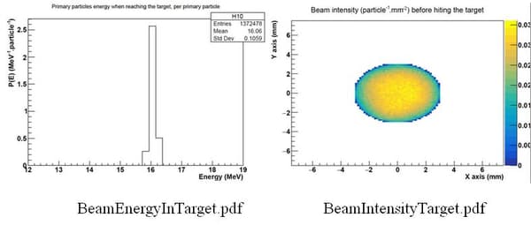
- BeamEnergyInFoil.pdf and BeamEnergyInTarget.pdf: beam energy distribution before entering the foil/target using histograms 1D0 and 1D1, normalised to the number of primary protons and the bin width.
- BeamEnergyOutFoil.pdf and BeamEnergyOutTarget.pdf: beam energy distribution when exiting the foil/target, using histograms 1D2 and 1D3, normalised to the number of primary protons and the bin width.
- BeamIntensityInFoil.pdf and BeamIntensityInTarget.pdf: beam intensity before entering the foil/target using histograms 2D0 and 2D1, normalised per primary particle and to the bins widths.
- BeamIntensityOutTarget.pdf: beam intensity when exiting the target using histogram 2D4, normalised per primary particle and to the bins widths.
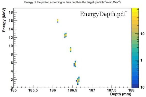
- EnergyDepth.pdf: energy of protons as a function of the depth in the target.
Example of outputs are shown here:
- Results/IsotopesProduction
- ActivityOfXX.pdf and YieldOfXX.pdf: Shows the production of the isotope XX (number of nuclei or activity) as a function of the time, starting from the beginning of irradiation and up to 30 hours. Note that if the time of irradiation is longer than 30 hours, you must change the maximum time to display the activity or yield by opening the file Plot.C and changing tMax.
- ActivitySaturationOfXX.pdf and YiedSaturationOfXX.pdf: Shows the saturation reached for the production of the isotope XX (number of nuclei or activity) as a function of the time, if the time of irradiation is set ‘infinite’.
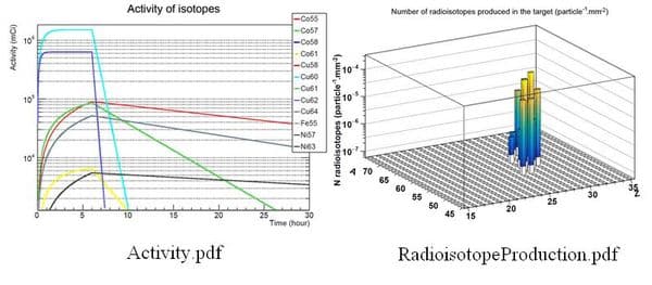
- Activity.pdf/Activity.jpg and Yield.pdf/Yield.jpg: Shows the activity (or yield) of all the isotopes produced during the irradiation as a function of the time up to 30 hours on the same graph.
- TotalActivity.pdf: Shows the sum of the activities induced by all the radioisotope up to 30 hours.
- RadioisotopeProduction.pdf/RadioisotopeProduction.jpg: Shows the number of isotopes produced per primary particles, as a function of Z and A.
- DepthCreation.pdf: Shows the depth at which radioisotopes were created.
An example of output is here below:
- ParticlesEnergySpectra folder
- Subfolder: beam. Energy spectra (normalized per primary particles and bin width) of particles created following the inelastic interaction of the beam with the target (1D 5->8).
- Subfolder: decay. Energy spectra (normalized per primary particles and bin width) of particles created following the decay of radioisotopes created in the target (1D 9->14).
Analysis of the results: verification and comparison to experimental data
The accuracy and consistency of the simulation results can be verified by checking the nuclear database you are using. You may refer to the following website : http://www.oecd-nea.org/janis/book/
In the web access part, click on the “protons” to access the database of protons. Click on the atomic species of the target. For example, for the production of Cu-64, Ni-64 is used, so you will click on 28-Ni. The list of isotopes of Nickel is available. Click on Ni-64 (Z=28) and select the nuclear reaction of interest. The cross sections will be displayed for different nuclear databases and experiments. The year of the nuclear databases displayed might be different from the one you are using. To display the ones used in the simulation, click on the following link: http://www.oecd-nea.org/janisweb/search/endf.
The computed values can be compared to experimental ones using the EXFOR website.
Last updated: 24/02/2022 by S. Guatelli