Advanced Example Xray_TESdetector
Responsible Geant4 Collaborator: Paolo Dondero, Swhard S.r.l, Genova, Italy.
Contributors: Ronny Stanzani (Swhard S.r.l, Genova, Italy)
Short description
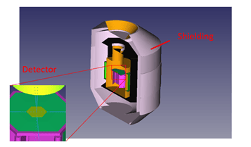
Xray_TESdetector is an example of the application of Geant4 in a space environment. It models an X-ray detector derived from the X-IFU, the X-ray spectrometer designed and developed by the European Space Agency (ESA) for use on the ATHENA telescope.
The detector is a Transition-edge sensor (TES) composed of 317 Bismuth pixels arranged in a hexagonal shape, and its setup includes different layers of shielding, filters and support.
The primary purpose of the simulation is to estimate the particle radiation background impacting the detector. For execution time optimization purposes, only particle steps respecting specific conditions (e.g. hit selected volumes close to the detector) are stored in a .root file [2]. An example of ROOT-based analysis of the output file is included (./analysis/analysis.C) and can be used to obtain basic plots and histograms.
Xray_TESdetector implements a physics list dedicated to space radiation interactions developed within the ESA AREMBES Project for the ATHENA mission, called Space Physics List (SPL).
Technically, this example shows how to manage a complex geometry obtained with advanced detector construction features (e.g., boolean operations and parameterization).
In addition, the example shows a method to optimize the simulation’s execution time and output size by selectively saving data based on specific combined conditions (e.g., position, eventID and process name).
Geometrical set-up
The geometry consists of a simplified version of the X-IFU detector and is composed of the following:
- the TES array, the backscattering (BSC) and the Anti-coincidence detector (ACD);
- the structural elements supporting the detector (e.g., the cage underneath it);
- the thermal shieldings;
- the structural elements of the cryostat chamber;
- a hollow Aluminum sphere schematizing the satellite.
Detector parameters:
- Detector thickness: 3 micrometers
- Number of pixels: 317
- Detector’s shape: regular hexagon
- Hexagon’s apothem: 8.593 mm
The default geometry is constructed in the DetectorConstruction class. Alternatively, a GDML file is provided (xray_TESdetector.gdml). The position of each pixel is defined by a list of coordinates (x,y) contained in pixelpos.txt.
Physics
The radiation field is composed of galactic cosmic rays (GCR) protons with a flux estimated for the L1/L2 Lagrangian points, as described in [1]. The energies range from 10 MeV to 100 GeV, and the particles are isotropically generated on the surface of a sphere surrounding the geometry and randomly launched toward its interior. The detector is placed in the sphere’s centre, and the sphere’s radius is chosen to avoid intersections with geometric elements.
This example implements a dedicated physics list called the Space Physics List, developed within the ESA AREMBES Project. This physics list has been designed to focus on the ATHENA physics processes but contains high-precision models that can be used in a more general space application. In detail, this physics list provides a custom electromagnetic part combined with the QBBC hadronic physics list. In volumes near the detector, where high precision in the scattering description is needed, using the Single Scattering (SS) model is recommended, as shown in run01.mac, through the SetEmRegion command. To have SS only in selected regions allows the simulation to reduce CPU consumption in most volumes and be very accurate near the detector. The default production cuts are selected for all volumes, i.e. 1 mm.
Simulation output
Xray_TESdetector provides an analysis macro example (analysis.C) with several predefined histograms:
- Average energy deposition per pixel (1D);
- Energy deposition on the detector (2D);
- Particle count per pixel (1D);
- Spectra of the primaries on the detector (1D);
- Total spectra on the detector (1D);
- Distribution of the particles on the detector (1D).
The first three are used to qualitatively check how the interactions are distributed on the detector pixels and what is the average energy deposition per pixel and particle type. The 2D histogram for the Energy deposit on the detector shows the detector’s shape on the XY plane. The spectra histograms are used to observe the following:
- the initial energies of the particles (at launch or generation);
- the energy deposit on the detector;
- the energy of the step before the impact on the pixel.
This information is the starting point to assess the radiation background composition and intensity of the detector, thus optimizing the detector shielding and background rejection techniques. Histograms are managed by the analysis.C file.
References
[1] S. Lotti, S. Molendi, C. Macculi, V. Fioretti, L. Piro et al., “Review of the Particle Background of the Athena X-IFU Instrument”, The Astrophysical Journal, 2021.
[2] BRUN, René, et al. “The ROOT Users Guide”. CERN, http://root.cern.ch, 2003.
Acknowlegements
Example developed within the ESA AREMBES Project, Contract n. 4000116655/16/NL/BW. This example is a reduced mass model of the Athena X-IFU instrument based on an early configuration which is no more applicable for any evaluation.
Last updated: 26/05/2023 by S. Guatelli